21 The measurement formula

As already mentioned, when viewing an object, the camera receives radiation not only from the object itself. It also collects radiation from the surroundings reflected via the object surface. Both these radiation contributions become attenuated to some extent by the atmosphere in the measurement path. To this comes a third radiation contribution from the atmosphere itself.

This description of the measurement situation, as illustrated in the figure below, is so far a fairly true description of the real conditions. What has been neglected could for instance be sun light scattering in the atmosphere or stray radiation from intense radiation sources outside the field of view. Such disturbances are difficult to quantify, however, in most cases they are fortunately small enough to be neglected. In case they are not negligible, the measurement configuration is likely to be such that the risk for disturbance is obvious, at least to a trained operator. It is then his responsibility to modify the measurement situation to avoid the disturbance e.g. by changing the viewing direction, shielding off intense radiation sources etc.

Accepting the description above, we can use the figure below to derive a formula for the calculation of the object temperature from the calibrated camera output.

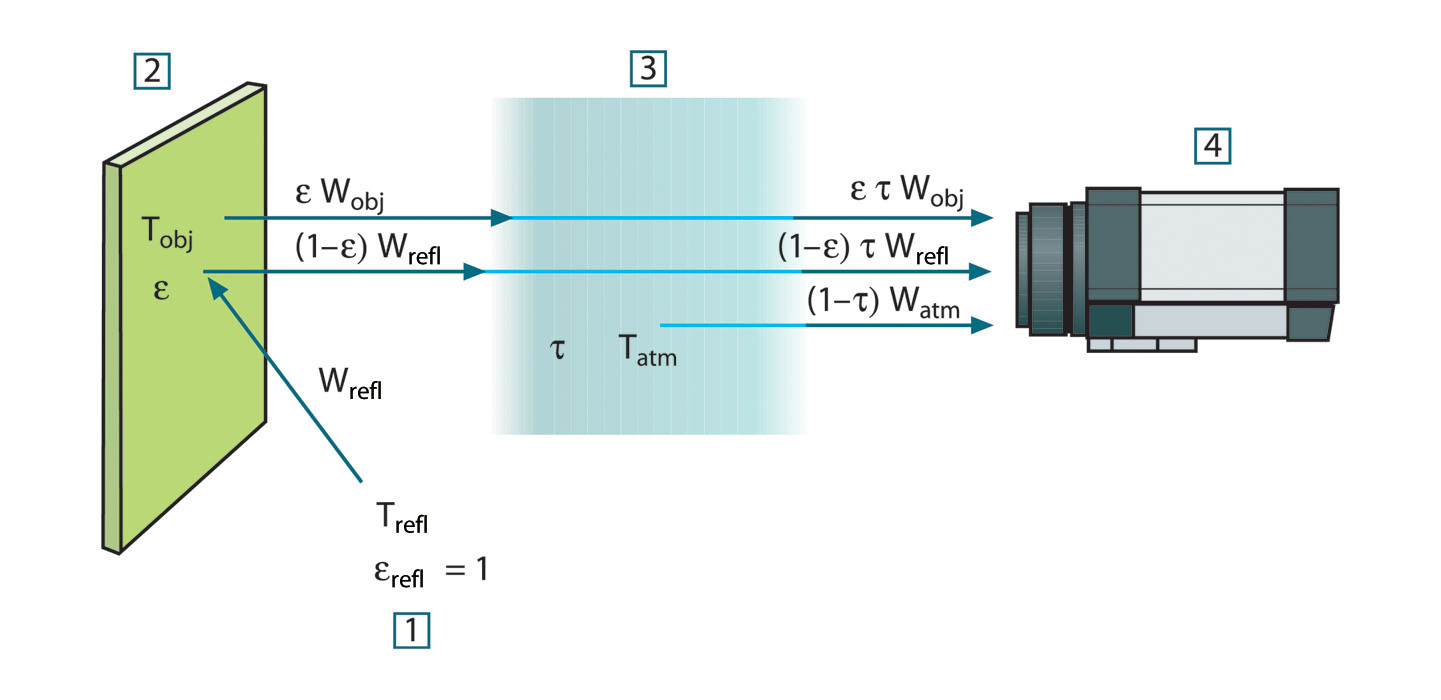
Figure 21.1 A schematic representation of the general thermographic measurement situation.1: Surroundings; 2: Object; 3: Atmosphere; 4: Camera

Assume that the received radiation power W from a blackbody source of temperature Tsource on short distance generates a camera output signal Usource that is proportional to the power input (power linear camera). We can then write (Equation 1):

or, with simplified notation:

where C is a constant.

Should the source be a graybody with emittance ε, the received radiation would consequently be εWsource .

We are now ready to write the three collected radiation power terms:

Emission from the object = ετWobj , where ε is the emittance of the object and τ is the transmittance of the atmosphere. The object temperature is Tobj .

Reflected emission from ambient sources = (1 – ε)τWrefl , where (1 – ε) is the reflectance of the object. The ambient sources have the temperature Trefl .

It has here been assumed that the temperature Trefl is the same for all emitting surfaces within the halfsphere seen from a point on the object surface. This is of course sometimes a simplification of the true situation. It is, however, a necessary simplification in order to derive a workable formula, and Trefl can – at least theoretically – be given a value that represents an efficient temperature of a complex surrounding.

Note also that we have assumed that the emittance for the surroundings = 1. This is correct in accordance with Kirchhoff’s law: All radiation impinging on the surrounding surfaces will eventually be absorbed by the same surfaces. Thus the emittance = 1. (Note though that the latest discussion requires the complete sphere around the object to be considered.)

Emission from the atmosphere = (1 – τ)τWatm , where (1 – τ) is the emittance of the atmosphere. The temperature of the atmosphere is Tatm .

The total received radiation power can now be written (Equation 2):

We multiply each term by the constant C of Equation 1 and replace the CW products by the corresponding U according to the same equation, and get (Equation 3):

Solve Equation 3 for Uobj (Equation 4):

This is the general measurement formula used in all the FLIR Systems thermographic equipment. The voltages of the formula are:

Table 21.1 Voltages

Uobj	Calculated camera output voltage for a blackbody of temperature Tobj i.e. a voltage that can be directly converted into true requested object temperature.
Utot	Measured camera output voltage for the actual case.
Urefl	Theoretical camera output voltage for a blackbody of temperature Trefl according to the calibration.
Uatm	Theoretical camera output voltage for a blackbody of temperature Tatm according to the calibration.

The operator has to supply a number of parameter values for the calculation:

the object emittance ε,
the relative humidity,
Tatm
object distance (Dobj )
the (effective) temperature of the object surroundings, or the reflected ambient temperature Trefl , and
the temperature of the atmosphere Tatm

This task could sometimes be a heavy burden for the operator since there are normally no easy ways to find accurate values of emittance and atmospheric transmittance for the actual case. The two temperatures are normally less of a problem provided the surroundings do not contain large and intense radiation sources.

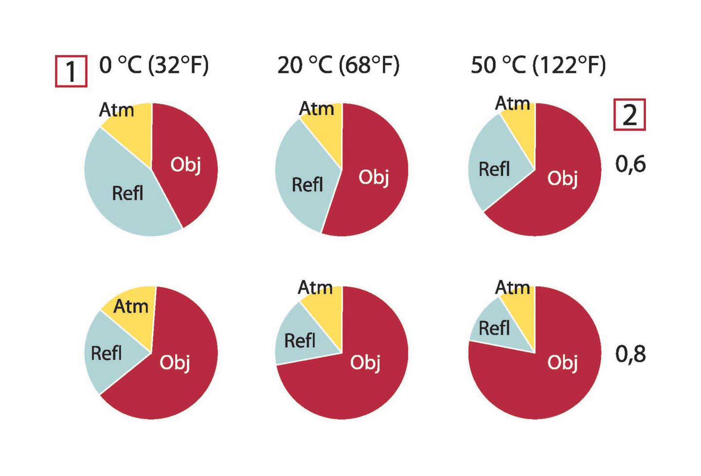
A natural question in this connection is: How important is it to know the right values of these parameters? It could though be of interest to get a feeling for this problem already here by looking into some different measurement cases and compare the relative magnitudes of the three radiation terms. This will give indications about when it is important to use correct values of which parameters.

The figures below illustrates the relative magnitudes of the three radiation contributions for three different object temperatures, two emittances, and two spectral ranges: SW and LW. Remaining parameters have the following fixed values:

τ = 0.88
Trefl = +20°C (+68°F)
Tatm = +20°C (+68°F)

It is obvious that measurement of low object temperatures are more critical than measuring high temperatures since the ‘disturbing’ radiation sources are relatively much stronger in the first case. Should also the object emittance be low, the situation would be still more difficult.

We have finally to answer a question about the importance of being allowed to use the calibration curve above the highest calibration point, what we call extrapolation. Imagine that we in a certain case measure Utot = 4.5 volts. The highest calibration point for the camera was in the order of 4.1 volts, a value unknown to the operator. Thus, even if the object happened to be a blackbody, i.e. Uobj = Utot , we are actually performing extrapolation of the calibration curve when converting 4.5 volts into temperature.

Let us now assume that the object is not black, it has an emittance of 0.75, and the transmittance is 0.92. We also assume that the two second terms of Equation 4 amount to 0.5 volts together. Computation of Uobj by means of Equation 4 then results in Uobj = 4.5 / 0.75 / 0.92 – 0.5 = 6.0. This is a rather extreme extrapolation, particularly when considering that the video amplifier might limit the output to 5 volts! Note, though, that the application of the calibration curve is a theoretical procedure where no electronic or other limitations exist. We trust that if there had been no signal limitations in the camera, and if it had been calibrated far beyond 5 volts, the resulting curve would have been very much the same as our real curve extrapolated beyond 4.1 volts, provided the calibration algorithm is based on radiation physics, like the FLIR Systems algorithm. Of course there must be a limit to such extrapolations.

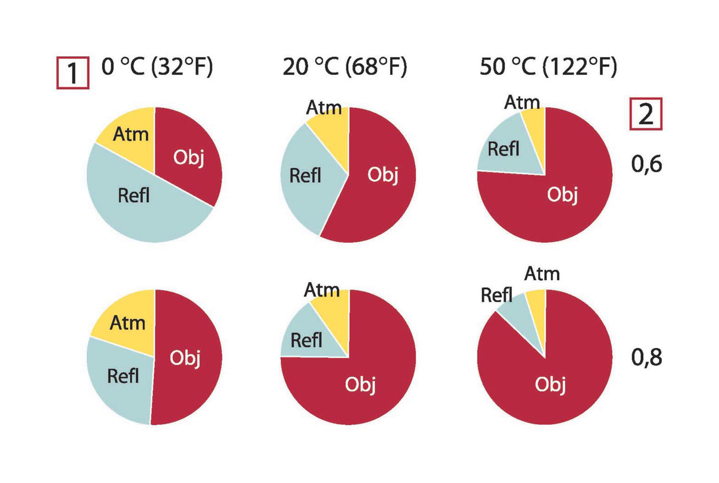
Figure 21.2 Relative magnitudes of radiation sources under varying measurement conditions (SW camera). 1: Object temperature; 2: Emittance; Obj: Object radiation; Refl: Reflected radiation; Atm: atmosphere radiation. Fixed parameters: τ = 0.88; Trefl = 20°C (+68°F); Tatm = 20°C (+68°F).

Figure 21.3 Relative magnitudes of radiation sources under varying measurement conditions (LW camera). 1: Object temperature; 2: Emittance; Obj: Object radiation; Refl: Reflected radiation; Atm: atmosphere radiation. Fixed parameters: τ = 0.88; Trefl = 20°C (+68°F); Tatm = 20°C (+68°F).